This report documents the annual water-year migration of depth-to-water observations, including ingestion of ZRXP data, QA/QC screening, integration with the active database, and preparation of OVGA-formatted deliverables.
Author
Inyo County Water Department
Published
October 1, 2025
Modified
January 26, 2026
Abstract
This report documents the annual processing and quality control of depth-to-water (DTW) observations from monitoring wells in the Owens Valley. The workflow ingests ZRXP-formatted data from LADWP, performs QA/QC screening, integrates observations with the active database, and generates OVGA-compliant deliverables for regional groundwater management.
Two key terms are used throughout: station identification (staid) for the unique well or sensor ID, and reference point elevation (RP elevation) for the fixed elevation from which depth is measured. Data are delivered as ZRXP text files, parsed and averaged to daily values per station, then filtered to retain only records with valid reference point elevations that correspond to OVGA-approved monitoring locations. Outputs include an annual update file, a consolidated master table, and upload-ready CSV files with accompanying plots and summary statistics for database import validation.
Annual update instructions: See ANNUAL_UPDATE_GUIDE.md for comprehensive step-by-step instructions on updating this workflow for the next water year.
Data sources and preprocessing
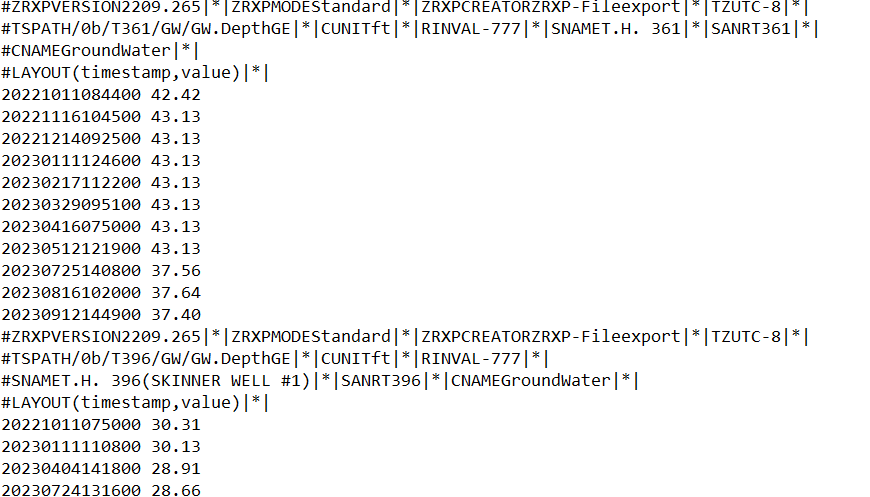
Here we load the raw data and combine it into one table. Each file is a text format (ZRXP): every monitoring point has a header line with its station identification (staid), followed by lines of date-and-value pairs. In R we (1) read each file, (2) pull the staid from the #TSPATH header, and (3) join the three files by staid and date so we have depth from reference point, depth below ground, and water surface elevation in one place.
Many stations record more than once per day. We later average those to one value per station per day so the dataset is smaller and all stations are on the same time step—that’s “daily harmonization.”
Input files (WY2025):
DepthRP_2024-25.dat — depth to water from reference point elevation (RP elevation)
DepthGE_2024-25.dat — depth to water below ground elevation
OwensValley_DepthWSE_2024-25.dat — water surface elevation
input data
# new data updates -------file_pathWSE <-here('data','hydro','2024-25 Water Year Transfer Packet for ICWD','OwensValley_DepthWSE_2024-25.dat')file_pathRP <-here('data','hydro','2024-25 Water Year Transfer Packet for ICWD','DepthRP_2024-25.dat')file_pathGE <-here('data','hydro','2024-25 Water Year Transfer Packet for ICWD','DepthGE_2024-25.dat')wYear <-'2025'parse_depth_file <-function(file_path, value_name) { dat_content <-readLines(file_path) data_list <-list() is_data_line <-function(line) {grepl("\\d+ \\d+\\.\\d+", line) }for (line in dat_content) {if (startsWith(line, "#TSPATH")) { staid <-sub('.*/([TVFRSW]\\w+).*', '\\1', line) }if (!startsWith(line, "#") &&is_data_line(line) &&!is.na(staid)) { data_list <-c(data_list, list(data.frame(staid, dateread = line))) } } data_df <-bind_rows(data_list) %>%select(staid, dateread) %>%na.omit() data_df <- data_df %>%separate(dateread, c("date", value_name), sep =" ") data_df[[value_name]] <-as.numeric(data_df[[value_name]]) data_df}depthRP_path <-here('data','hydro','2025','depthRP.RDS')depthGE_path <-here('data','hydro','2025','depthGE.RDS')depthWSE_path <-here('data','hydro','2025','depthWSE.RDS')depthRP <-if (file.exists(depthRP_path)) {readRDS(depthRP_path)} else { depthRP <-parse_depth_file(file_pathRP, "dtw.rp")saveRDS(depthRP, file = depthRP_path) depthRP}depthGE <-if (file.exists(depthGE_path)) {readRDS(depthGE_path)} else { depthGE <-parse_depth_file(file_pathGE, "dtw.bgs")saveRDS(depthGE, file = depthGE_path) depthGE}depthWSE <-if (file.exists(depthWSE_path)) {readRDS(depthWSE_path)} else { depthWSE <-parse_depth_file(file_pathWSE, "wse")saveRDS(depthWSE, file = depthWSE_path) depthWSE}# ground surface elevation at staidsgse_staids <-read_csv(here('data','hydro', 'gse_staids.csv'))# staids in ovga database------# used to cross reference what will be accepted into an import# need to filter out staids that aren't in the ovga list, otherwise import will fail# Latest monitoring points (if updated): https://owens.gladata.com/api/export.ashx?v=mp (may require authentication; save as Owens_Monitoring_Points.csv)ovga_points <-read_csv(here("data","hydro","Owens_Monitoring_Points.csv"))# If JSON export exists, load as alternate list for "now on new list" summary and optional useovga_points_from_json <-NULLif (file.exists(here("data","hydro","owens_mp_export.json"))) { mp_json <- jsonlite::fromJSON(here("data","hydro","owens_mp_export.json")) need <-c("mon_pt_id", "site_id", "mon_pt_name", "mon_pt_lat", "mon_pt_long", "coord_sys", "county")if (all(need %in%names(mp_json))) { ovga_points_from_json <- mp_json %>%select(all_of(need))if (!"hide_from_public"%in%names(mp_json)) ovga_points_from_json$hide_from_public <-0Lelse ovga_points_from_json$hide_from_public <-as.integer(mp_json$hide_from_public) }}# reference point elevation - some staids don't have RP elevations. Identify these here for the current water year transferrpelev <-read_csv(here('data','hydro','rp_elev.csv'))last_ovga_mw <-read_csv(here('output','ovga_uploads_mw_with_rpe_102023_092024_zn.csv'))# historical water levels------hist <-read_csv(here('output','Monitoring_Wells_Master_2024.csv'))hist$date <-ymd(hist$date)
Raw input coverage
The table below provides a quick inventory of each input file: record counts, unique monitoring points, and the raw date range. Use this to verify that the received transfer packet aligns with expectations before moving on to joins, aggregation, and exports.
File
Records
Unique_staids
Date_start
Date_end
DepthRP_2024-25.dat
82831
743
2024-10-01
2025-09-30
DepthGE_2024-25.dat
74670
655
2024-10-01
2025-09-30
OwensValley_DepthWSE_2024-25.dat
86968
383
2024-10-01
2025-09-30
Each file repeats headers for each monitoring well. Extract the well ID from #TSPATH and join to observation rows (lines that do not start with #). The example shows the header block followed by timestamped values.
Data combination and daily harmonization
testwellupdate
# rename the columns# clean up the date with formal date specificationtestwell.up <- try %>%select(-date, -datetime) %>%rename(date = date.y.m.d) %>%mutate(source ="DWP") # head(testwell.up)
append updates to master database
## Append updates to mastertestwells.combined <-bind_rows(hist, testwell.up) # head(testwells.combined)# 1,145,360 records going back to 1971# testwells.combined %>% n_distinct(staid)# testwells.combined %>% distinct(staid) %>% nrow()
Metric
Value
Annual update rows
89,289
Annual update staids
750
Active database rows
1,324,540
Active database staids
1,381
ICWD database refresh
This section appends the annual update to the internal (ICWD) master database, writes the yearly slice and refreshed master to output/2025wy/ICWD, and provides a preview of the update table for review. A full-resolution (pre-daily aggregation) extract is also written to preserve all raw reads for archive and troubleshooting.
At this stage the annual update (testwellwy2025.csv) represents the daily harmonized water-year slice, while the master database output (Monitoring_Wells_Master_2025.csv) provides the full historical record with the new year appended. These outputs are the authoritative internal datasets used for QA/QC, reporting, and follow-on exports.
testwellwy2025.csv is the WY2025 daily slice (one row per station per day). testwellwy2025_raw.csv keeps every read before daily averaging, for archive or troubleshooting.
Depth-to-water is measured from a fixed mark at each well—the reference point elevation (RP elevation). We need that value to interpret the depth numbers. In this section we attach the most recent reference point elevation to each station id(entification) (staid) and flag any stations where it’s missing.
Stations without a reference point elevation stay in our internal tables but are left out of the OVGA upload so we don’t import incomplete records. We still keep the data for later if RP values are added.
First we convert the RP dates into a standard format so we can join them to the annual update.
convert RP dates
## RP can be continually changing so need to be recursive with the RP file for updates.# date conversionrpelev_date <- rpelev %>%mutate(date = lubridate::mdy(date_c))head(rpelev_date) %>%datatable(options =list(pageLength =10, lengthChange =TRUE, scrollX =TRUE))
Next, we identify the most recent reference point elevation per staid. That way each monitoring point uses the latest available reference point during the update.
We then attach that most recent reference point elevation to each staid so every row has a reference point value for the join.
We join RP elevations to the annual update so DTW values can be expressed relative to the reference point. This join also supports QA/QC checks for missing RP data.
count_unique_staids
1 750
After the reference-point join we average to one value per station per day. OVGA accepts no more than one value per station per day, so this daily aggregation is required for the OVGA import. For staids with many readings per day we take the mean; that also keeps the table smaller and every staid on the same time step.
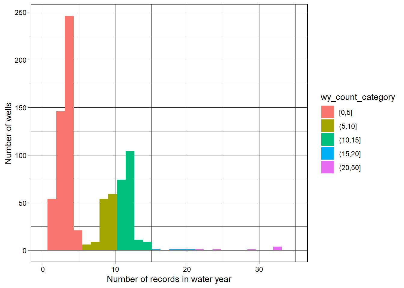
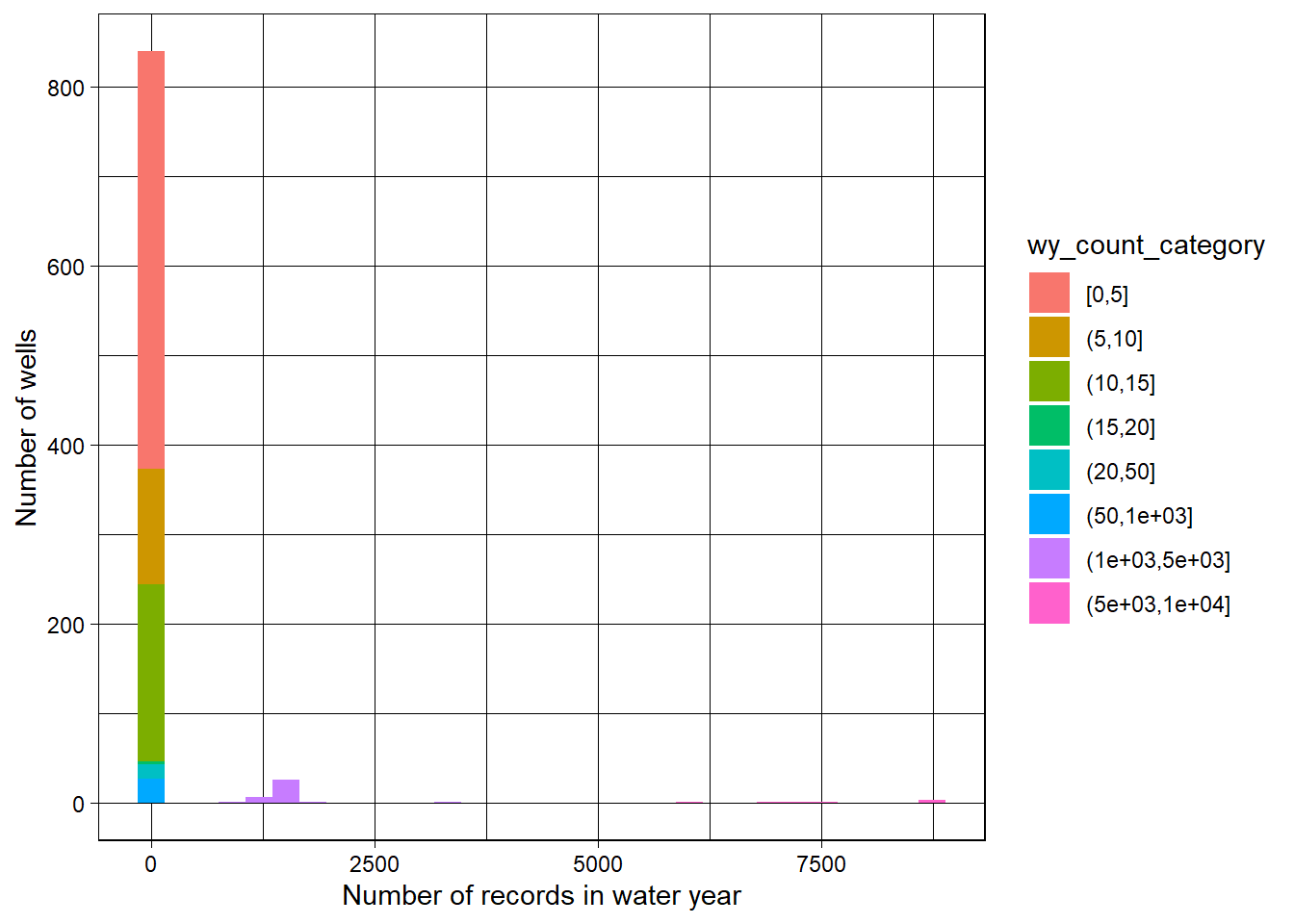
The tables and plots below summarize measurement frequency and daily aggregation behavior, which is used to validate that the daily rollup is behaving as expected.
WY2025 update: 33 out of 750 staids have multiple measurements per day (some hourly and a few up to 15‑minute intervals). 32 of those 33 staids also have single‑measurement days.
We harmonize these to daily values to reduce data size and make the annual update consistent across measurement frequencies. The next steps show how we aggregate to daily means and then summarize record frequency by water year to confirm that high-frequency sensors are behaving as expected.
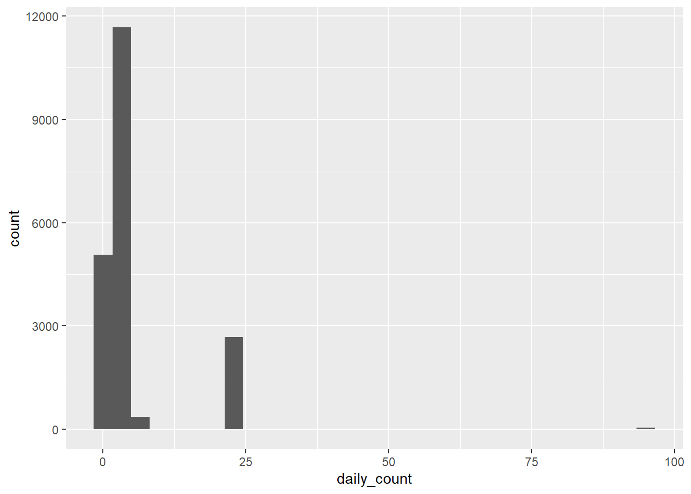
The distributions below provide a QA/QC snapshot of record counts per staid. A small subset of sites should show high counts (automated sensors), while most sites should fall in the low-frequency bins (manual measurements).
Daily averaging collapses multiple measurements on the same day to a single value per staid and day. This daily series is the basis for annual summaries and export preparation.
We also infer a measurement method flag based on measurement frequency so that OVGA export metadata stays consistent when explicit method values are not provided with the raw data.
assign TR vs ES method based on measurement frequency
# More than 4 reads per month (48 per year) indicates pressure transducer (TR);# fewer indicates electric sounder (ES).record.number <- dtwrp.rpelev %>%filter(!is.na(rp_elev)) %>%group_by(staid) %>%summarise(count.with.rpe =n()) %>%mutate(MMethod =case_when(count.with.rpe >=48~"TR", count.with.rpe <48~"ES"))# if there are four reads per day, once per month, approximates to 48. quick and dirty separation. a list of pressure transducer staids would be better if it could be maintained.head(record.number %>%arrange(-count.with.rpe))
# records per staidLA.staids <- dtwrpavg.rpelev %>%group_by(staid) %>%summarise(records =n())# head(LA.staids)# LA.staids %>% arrange(desc(records))#785
The next QA/QC steps narrow the dataset to records eligible for OVGA import. We first identify staids that are present in the OVGA monitoring-point list, then quantify which of those lack RP elevations. Finally, we filter to records with valid RP elevations and OVGA-listed points before building the export template.
staids in data that are also on ovga list
LA.staids.in.ovga <- LA.staids %>%semi_join(ovga_points, by =c("staid"="mon_pt_name"))# LA.staids.in.ovga %>% nrow()#714
monitoring points missing rp elevations after join
# monitoring points missing rp elevations after join# LA.staids.in.ovga# find how many staids are missing rp elevationna.rp.elev <- dtwrpavg.rpelev %>%semi_join(LA.staids.in.ovga, by ='staid') %>%filter(is.na(rp_elev)) %>%group_by(staid) %>%summarise(count.na =n())
anti_join take NA rp elev off
# anti_join removes records in x that match y# Select only data with rp elevations (not na)rpselect <- dtwrpavg.rpelev %>%anti_join(na.rp.elev, by ="staid")# rpselect# 19,793 1.24.2024
Filter to records with RP elevation and valid OVGA monitoring points.
semi_join retain records in ovga staid list
# 6,048 points including monitoring wells, pumping wells, surface water gauging stations.# semi_join returns records in x with a match in yrpselect2 <- rpselect %>%semi_join(ovga_points, by =c("staid"="mon_pt_name"))# head(rpselect2)rpselect2 %>%arrange(staid,desc(date))
The upload file for OVGA is built from the daily table after we drop rows that don’t belong: we keep only stations on the OVGA list, only rows that have a valid reference point elevation, and only depth values that pass our checks (not missing, not -777, not ≥ 500 ft). What’s left is a clean table that matches the OVGA import template.
Column names and order follow that template so the system can ingest the file without errors. The file is saved under output/2025wy/OVGA and used for the actual import.
# OVGA Import Depth to Water: columns per schema (ReportingDate and UseInReporting optional; blank ReportingDate uses DateMeasured)ovga_dtw_cols <-c("WellName", "DateMeasured", "ReportingDate", "DepthToWater", "ReferencePointElevation", "QAQCLevel", "MeasMethod", "NoMeasFlag", "QuestMeasFlag", "DataSource", "CollectedBy", "UseInReporting", "Notes")write_ovga_dtw_csv <-function(x, path) {# Drop any staid/date so only OVGA-named columns (WellName, DateMeasured, ...) are written x <- x %>%select(-any_of(c("staid", "date"))) %>%select(all_of(ovga_dtw_cols)) x[] <-lapply(x, function(v) ifelse(is.na(v), "", as.character(v)))write.table(x, path, sep =",", row.names =FALSE, quote =FALSE)}out_ovga <-here("output", "2025wy", "OVGA")dir.create(out_ovga, recursive =TRUE, showWarnings =FALSE)write_ovga_dtw_csv(upload, file.path(out_ovga, "ovga_uploads_mw_with_rpe_102024_092025_zn.csv"))writexl::write_xlsx(upload %>%select(-any_of(c("staid", "date"))) %>%select(all_of(ovga_dtw_cols)) %>%mutate(across(everything(), ~replace(., is.na(.), ""))), file.path(out_ovga, "ovga_uploads_mw_with_rpe_102024_092025_zn.xlsx"))
datatable
col_w <-list(list(targets =0:4, width ="80px"),list(targets =5, width ="100px"),list(targets =6:10, width ="90px"))datatable( upload,caption ="2024-2025 water year upload formatted for OVGA data management system.",options =list(pageLength =10,lengthChange =TRUE,scrollX =TRUE,autoWidth =FALSE,columnDefs = col_w ),class ="compact stripe")
Metric
Value
Rows in OVGA upload
5515
Unique monitoring points
590
Date range
2024-10-01 to 2025-09-30
OVGA DTW exclusions (download)
Table 1: Staids not in OVGA monitoring points list
These staids are excluded because they are not on the current OVGA monitoring points list. This list should be reviewed by the hydrologist and DB manager to decide which staids should be added to the OVGA monitoring points list on the backend.
Table 2: Staids on OVGA list needing data quality resolution
These staids are on the OVGA monitoring points list but are excluded due to data quality issues. The “Missing reference point elevation” category excludes staids that received WSE-estimated RP (those 358 records were imported).
Exclusions summary
The exclusions are now split into two separate tables and export files for hydrologist handoff:
Table 1 (Not in OVGA list): 75 staids that are not on the current OVGA monitoring points list. These should be reviewed by the hydrologist and DB manager to decide which should be added to the OVGA backend.
Table 2 (Data quality issues): 49 exclusion entries for staids that are on the OVGA list but excluded for data quality reasons (missing reference point elevation, invalid depth, or invalid RP elevation). The “Missing RP” category in Table 2 excludes staids that received WSE-estimated RP—those were imported via the WSE-estimate-only file (358 records).
OVGA DTW exclusions by reason (WY2025). Table 2 Missing RP excludes WSE-estimated staids.
Exclusion reason
Unique staids
Total records
Note
Not in OVGA monitoring points list
75
3745
Table 1: For hydrologist/DB manager backend list review
Invalid depth (NA, -777, or >= 500 ft)
12
69
Table 2: Data quality issue
Missing reference point elevation
37
392
Table 2: Staids needing RP (WSE-estimated staids excluded)
Key outputs and datasets (output/2025wy/OVGA/):
OVGA DTW export files and record counts (WY2025).
Output
CSV
XLSX
Records / staids
Main OVGA DTW upload (reported RP only)
ovga_uploads_mw_with_rpe_102024_092025_zn.csv
ovga_uploads_mw_with_rpe_102024_092025_zn.xlsx
5,515
WSE-estimate-only upload (estimated RP)
ovga_uploads_wy2025_wse_estimate_only.csv
ovga_uploads_wy2025_wse_estimate_only.xlsx
358 (imported)
Table 1: Not in OVGA list
ovga_excl_not_in_list_wy2025.csv
ovga_excl_not_in_list_wy2025.xlsx
75 staids
Table 2: Data quality issues
ovga_excl_data_quality_wy2025.csv
ovga_excl_data_quality_wy2025.xlsx
49 exclusions
Combined exclusions (all reasons)
ovga_dtw_exclusions_wy2025.csv
ovga_dtw_exclusions_wy2025.xlsx
124 exclusion rows
RP elevation candidates (WSE+DepthRP)
rp_elev_candidates_wse_plus_dtw_wy2025.csv
rp_elev_candidates_wse_plus_dtw_wy2025.xlsx
40 staids
RP elevation with sources (reported vs estimated)
rp_elev_with_sources_wy2025.csv
rp_elev_with_sources_wy2025.xlsx
—
Table 2 contains 49 unique staids that are on the OVGA list but excluded for data quality reasons (missing RP, invalid depth, or invalid RP). Note that the “Missing RP” category in Table 2 excludes staids that received WSE-estimated RP elevation—those were successfully imported via the WSE-estimate-only file (358 records).
The staids excluded for missing reference point elevation in the original analysis that had sufficient WSE and DepthRP overlap were given estimated RP elevations (see Potential RP elevations derived from WSE + DepthRP in Appendix (with QA/QC)). These staids were imported via the WSE-estimate-only upload file (358 records accepted by OVGA). They no longer appear in Table 2’s “Missing RP” category because they were successfully resolved.
0 of 37 staids excluded for missing reference point elevation can get an estimated RP from WSE + DepthRP: ****.
Summary: exclusions “not on OVGA list” that are now on the updated monitoring points list
If you have refreshed the monitoring points list from the GLA API export, the following staids were excluded because they were not on the old list but are on the new list. After updating Owens_Monitoring_Points.csv and re-running the report, they would no longer be excluded for that reason.
6 of 75 staids excluded for not being on the OVGA list are on the updated monitoring points export: T977, T978D, T978S, V137, W426, W428. (If the JSON export has not been refreshed, this shows the last known set.)
Staids not on OVGA list (handoff for backend)
The following staids are excluded from the OVGA DTW upload because they are not on the current OVGA monitoring points list. This list is provided to the hydrologist and DB manager to decide on adding these staids to the OVGA monitoring points list on the backend. Once added, they can be included in future uploads.
The WY2025 depth-to-water import to OVGA completed successfully (358 records imported). Exclusions are documented above: staids on the OVGA list but excluded for data-quality reasons (missing RP, invalid depth/RP), and staids not on the OVGA list. The not-on-list staids are highlighted above for handoff to the hydrologist and DB manager to decide on adding them to the OVGA monitoring points list on the backend.
Record attrition by step
The table below summarizes how many records remain after each processing step. Raw reads are joined to reference point elevation, averaged to daily, then filtered to OVGA list and valid depth and RP so the final upload is a subset of the original.
WY2025 DTW record attrition by processing step.
Step
Records
stringsAsFactors
Percent_of_raw
Raw reads (all timestamps)
89,289
FALSE
100%
DTW with RP joined (pre-daily)
89,289
FALSE
100%
Daily DTW (post-aggregation)
10,079
FALSE
11.3%
Daily DTW in OVGA list
6,334
FALSE
7.1%
Daily DTW with RP elevation
5,643
FALSE
6.3%
Final OVGA upload
5,515
FALSE
6.2%
Appendix (with QA/QC)
GLA Data Depth to Water Import Procedures
Last verified in prior annual update; re-check against current OVGA guidance when preparing a new upload.
GLA Data Web application. The uploaded Excel Workbook must contain one spreadsheet with 13 columns with the following names in this order:
Field Name
Data Type
Required
WellName
Text
Yes
DateMeasured
Date
Yes
ReportingDate
Date
No
DepthToWater
Numeric
Conditional
ReferencePointElevation
Numeric
Conditional
QAQCLevel
Text
Yes
MeasMethod
Text
Yes
NoMeasFlag
Text
Conditional
QuestMeasFlag
Text
No
DataSource
Text
Yes
CollectedBy
Text
No
UseInReporting
Text
No
Notes
Text
Conditional
WellName The WellName column is required and must contain the name of a monitoring point within the basin selected when the file was uploaded.
DateMeasured The DateMeasured column is required. The field must be a date and can not be in the future nor more than 100 years in the past.
2-1-1 import error says that ReportingDate is not part of the column list ReportingDate The ReportingDate column must be blank or a date. If the field is a date, it must be within 14 days of DateMeasured. If left blank, the column is populated with the value in the DateMeasured column. This field allows users to assign a measurement to an adjacent month for reporting purposes. For example, a measurement collected on May 31st may be intended to be used as an April measurement.
DepthToWater This column must be blank or numeric. DepthToWater is the number of feet from the reference point. If blank, NoMeasFlag is required and ReferencePointElevation must also be blank. Positive values indicate the water level is below the top of the casing, while negative values indicate the water level is above the top of the casing (flowing artesian conditions).
ReferencePointElevation This column must be blank or numeric. ReferencePointElevation is the elevation in feet from where the depth to water measurement took place. If blank, NoMeasFlag is required and DepthToWater must also be blank.
QAQCLevel This field is required and must be one of the following values:
High - Data are of high quality
Medium - Data are inconsistent with previous values or sampling conditions were not ideal. Values will be displayed with a different color on plots.
Low - Data are not considered suitable for display or analysis due to inconsistencies with previous values or poor sampling conditions. Preserves sample in database for record-keeping purposes but not displayed on figures, tables, or used in analyses.
Undecided - QA/QC level has not been determined.
MeasMethod This field is required and must be one of the following values:
Code
Description
ES
Electric sounder measurement
ST
Steel tape measurement
AS
Acoustic or sonic sounder
PG
Airline measurement, pressure gage, or manometer
TR
Electronic pressure transducer
OTH
Other
UNK
Unknown
NoMeasFlag This field must be blank if DepthToWater and ReferencePointElevation contain values. Otherwise, this field is required and must be one of the following values:
Code
Description
0
Measurement discontinued
1
Pumping
2
Pump house locked
3
Tape hung up
4
Can’t get tape in casing
5
Unable to locate well
6
Well has been destroyed
7
Special/other
8
Casing leaking or wet
9
Temporary inaccessible
D
Dry well
F
Flowing artesian
QuestMeasFlag This field must be blank or be one of the following values:
Code
Description
0
Caved or deepened
1
Pumping
2
Nearby pump operating
3
Casing leaking or wet
4
Pumped recently
5
Air or pressure gauge measurement
6
Other
7
Recharge or surface water effects near well
8
Oil or foreign substance in casing
9
Acoustical sounder
E
Recently flowing
F
Flowing
G
Nearby flowing
H
Nearby recently flowing
DataSource This field is required and used to identify where the water level data came from (e.g., entity, database, file, etc.). Limit is 100 characters. default = “LADWP”
CollectedBy This field is optional and used to identify the person that physically collected the data. Limit is 50 characters. default = “LADWP”
UseInReporting This field is optional and used to filter measurements used in reports. If included, the value must be “yes”, “no”, “true”, “false”, “1” or “0”. If blank, a value of “yes” is assumed. default = “yes”
Notes This field must be populated if NoMeasFlag is 7 (special/other) or QuestMeasFlag is 6 (other), otherwise this field is optional. Limit is 255 characters. default = “blank”
OVGA DTW record density (north to south)
These maps show where records are concentrated north to south for the OVGA DTW upload and for excluded records. Point size scales with record counts. If the ggExtra package is available, a marginal density curve is added to highlight the north-south distribution.
OVGA DTW upload records with north-south density (size scales with record count).
OVGA DTW excluded records with north-south density (size scales with record count).
QA/QC and hydrographs
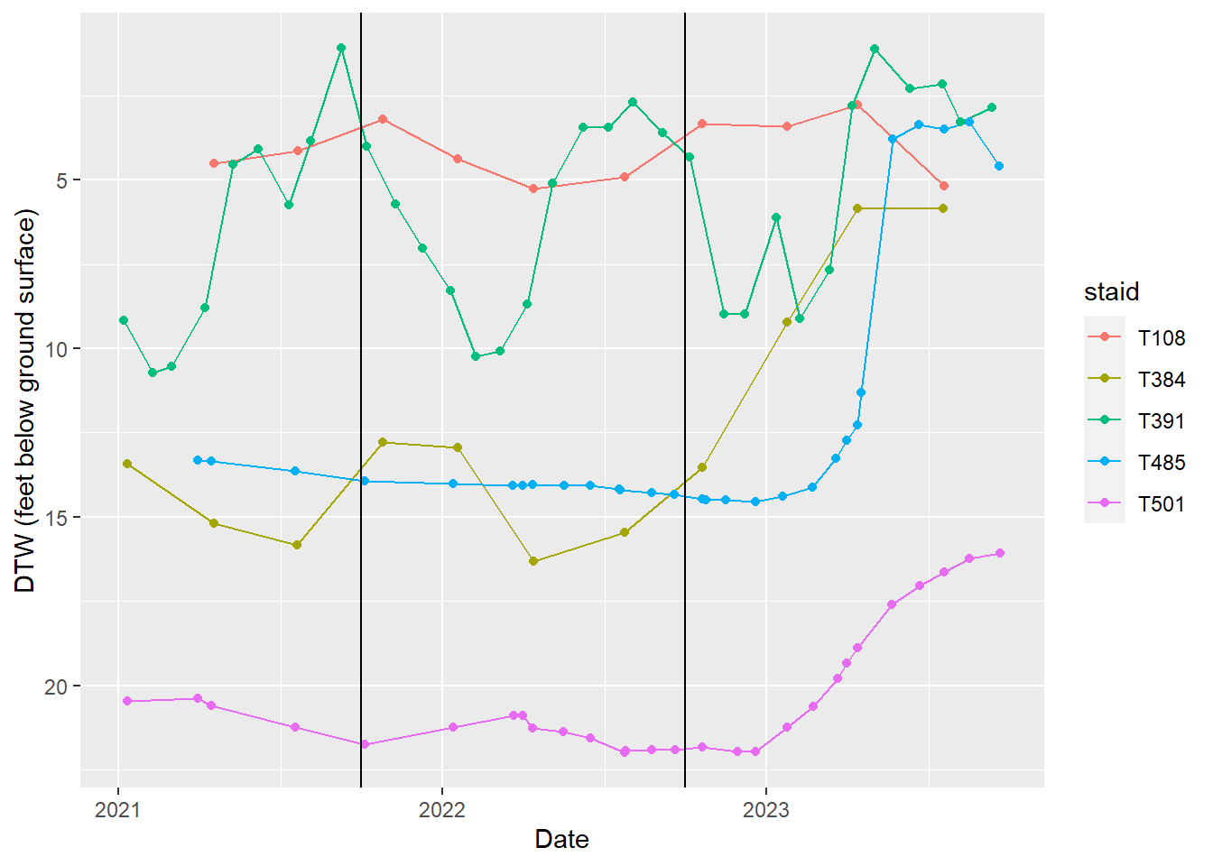
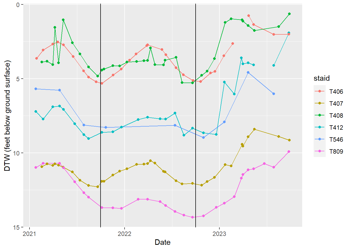
In this section we do two things: look at hydrographs (time-series plots of depth to water by well) and run automated checks. Hydrographs let you spot sudden shifts or odd patterns; the checks confirm record counts, missing reference point elevation, and that we only export station IDs that are on the OVGA list. Vertical lines on the plots mark water-year boundaries.
Laws wellfield
Hydrographs of indicator wells in the Laws wellfield.
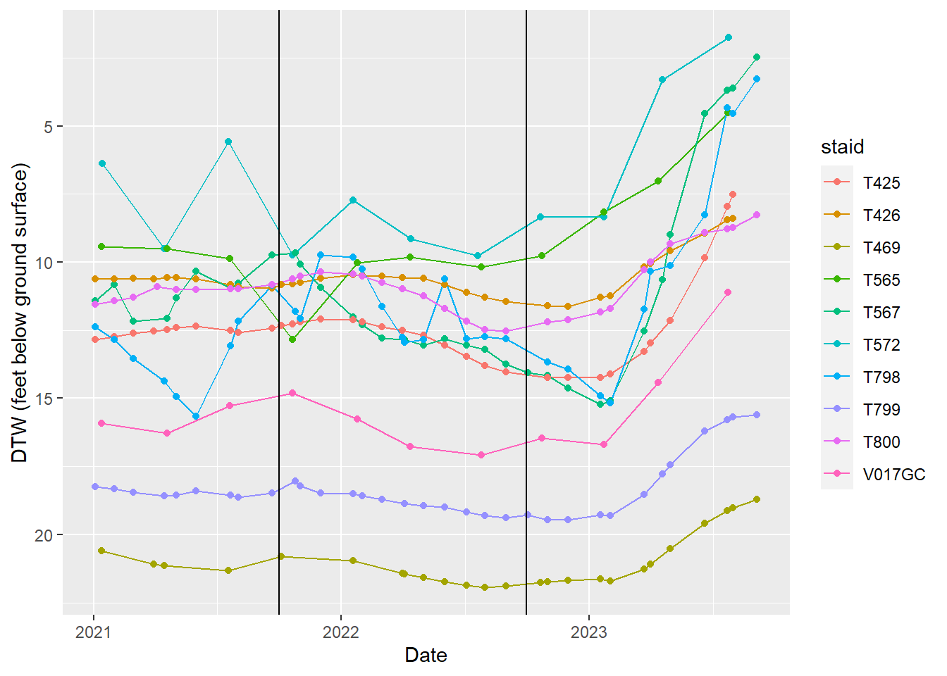
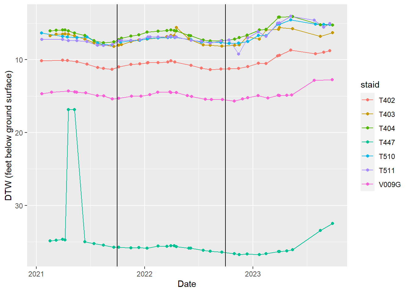
Bishop wellfield
Hydrographs of indicator wells in the Bishop wellfield.
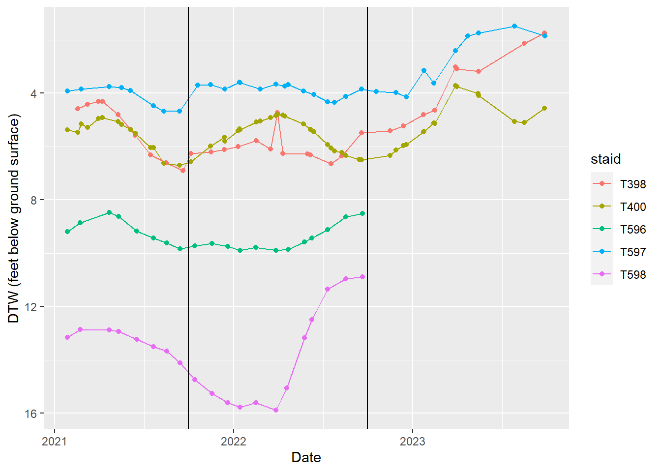
Big Pine wellfield
Hydrographs of indicator wells in the Big Pine wellfield. T565, and V017GC are in south Big Pine near W218/219.
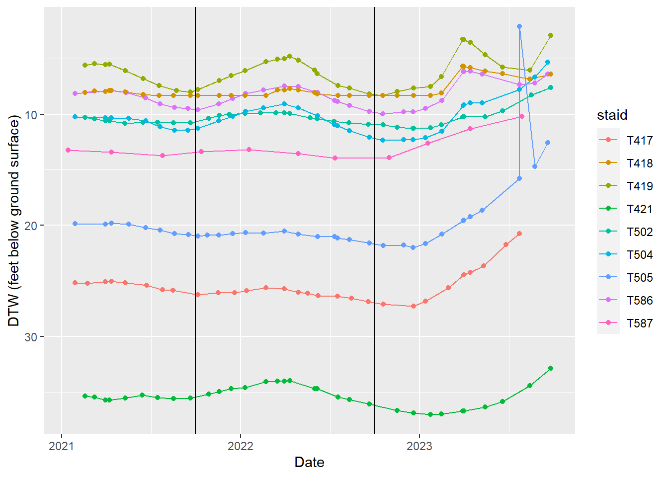
Taboose-Aberdeen wellfield
Hydrographs of indicator wells in the Taboose-Aberdeen wellfield.
Thibaut-Sawmill wellfield
Hydrographs of indicator wells in Thibaut-Sawmill wellfield.
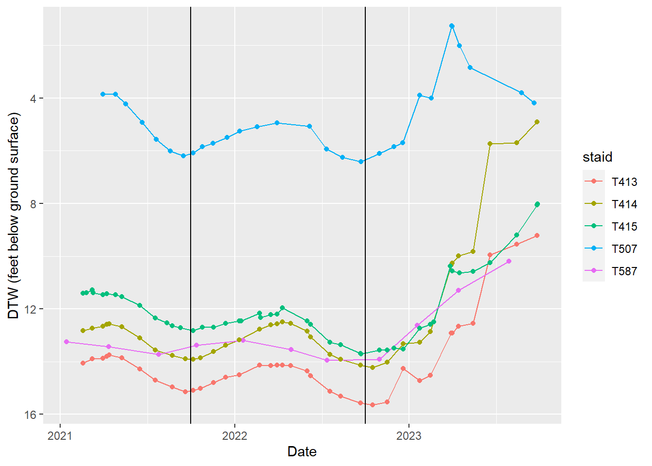
Independence-Oak wellfield
Hydrographs of indicator wells in Independence-Oak wellfield.
Symmes-Shepherd wellfield
Hydrographs of indicator wells in Symmes-Shepherd wellfield.
Bairs-George wellfield
Hydrographs of indicator wells in Bairs-George wellfield.
Citation
BibTeX citation:
@report{county_water_department2025,
author = {County Water Department, Inyo},
publisher = {Inyo County Water Department},
title = {Water {Levels} and {Depth} to {Water}},
date = {2025-10-01},
url = {https://inyo-gov.github.io/hydro-data/},
langid = {en}
}
For attribution, please cite this work as:
County Water Department, Inyo. 2025. “Water Levels and Depth to
Water.”Data Report. Inyo County Water Department. https://inyo-gov.github.io/hydro-data/.
Source Code
---title: "Water Levels and Depth to Water"subtitle: "Inyo County, California"description: "This report documents the annual water-year migration of depth-to-water observations, including ingestion of ZRXP data, QA/QC screening, integration with the active database, and preparation of OVGA-formatted deliverables."format: html: toc: true toc-depth: 4 anchor-sections: true smooth-scroll: true code-fold: true code-summary: "code" code-line-numbers: true code-overflow: wrap code-link: true html-math-method: katextbl-cap-location: top # number-sections: true author: "Inyo County Water Department"affiliation: "Inyo County Water Department"affiliation-title: "Senior Scientist"date: "2025-10-01"date-modified: "2026-01-26"draft: falseimage: "lw-i85-fac-1.png"citation: type: report container-title: "Data Report" publisher: "Inyo County Water Department" issued: "2025-10-01" url: https://inyo-gov.github.io/hydro-data/google-scholar: truecategories: [R, hydrology, monitoring wells, surface water flow, pumping volumes, LADWP data, OVGA, time series]---# AbstractThis report documents the annual processing and quality control of depth-to-water (DTW) observations from monitoring wells in the Owens Valley. The workflow ingests ZRXP-formatted data from LADWP, performs QA/QC screening, integrates observations with the active database, and generates OVGA-compliant deliverables for regional groundwater management.Two key terms are used throughout: **station identification (staid)** for the unique well or sensor ID, and **reference point elevation (RP elevation)** for the fixed elevation from which depth is measured. Data are delivered as ZRXP text files, parsed and averaged to daily values per station, then filtered to retain only records with valid reference point elevations that correspond to OVGA-approved monitoring locations. Outputs include an annual update file, a consolidated master table, and upload-ready CSV files with accompanying plots and summary statistics for database import validation.For a new water year, update the `year` variable in three locations: [input paths and master](#updatewy), [ICWD output file names](#masterdb), and [OVGA upload](#ovgaupdate). The full R workflow and report source are available in [index.qmd](https://github.com/inyo-gov/hydro-data/blob/main/index.qmd).**Annual update instructions:** See [ANNUAL_UPDATE_GUIDE.md](https://github.com/inyo-gov/hydro-data/blob/main/ANNUAL_UPDATE_GUIDE.md) for comprehensive step-by-step instructions on updating this workflow for the next water year.```{r packages-setup, warning = FALSE,message = FALSE,include=FALSE}#| code-fold: true#| code-summary: "packages"library(tidyverse)library(lubridate)library(readxl)library(writexl)library(knitr)library(here)library(DT)knitr::opts_chunk$set(echo =FALSE,warning =FALSE,message =FALSE,cache=FALSE)```# Data sources and preprocessing {#updatewy}Here we load the raw data and combine it into one table. Each file is a text format (ZRXP): every monitoring point has a header line with its **station identification (staid)**, followed by lines of date-and-value pairs. In R we (1) read each file, (2) pull the staid from the `#TSPATH` header, and (3) join the three files by staid and date so we have depth from reference point, depth below ground, and water surface elevation in one place.Many stations record more than once per day. We later average those to one value per station per day so the dataset is smaller and all stations are on the same time step—that’s “daily harmonization.”Input files (WY2025):- `DepthRP_2024-25.dat` — depth to water from **reference point elevation (RP elevation)**- `DepthGE_2024-25.dat` — depth to water below ground elevation- `OwensValley_DepthWSE_2024-25.dat` — water surface elevation```{r readdata, echo=TRUE}#| code-fold: true#| code-summary: "input data"# new data updates -------file_pathWSE <-here('data','hydro','2024-25 Water Year Transfer Packet for ICWD','OwensValley_DepthWSE_2024-25.dat')file_pathRP <-here('data','hydro','2024-25 Water Year Transfer Packet for ICWD','DepthRP_2024-25.dat')file_pathGE <-here('data','hydro','2024-25 Water Year Transfer Packet for ICWD','DepthGE_2024-25.dat')wYear <-'2025'parse_depth_file <-function(file_path, value_name) { dat_content <-readLines(file_path) data_list <-list() is_data_line <-function(line) {grepl("\\d+ \\d+\\.\\d+", line) }for (line in dat_content) {if (startsWith(line, "#TSPATH")) { staid <-sub('.*/([TVFRSW]\\w+).*', '\\1', line) }if (!startsWith(line, "#") &&is_data_line(line) &&!is.na(staid)) { data_list <-c(data_list, list(data.frame(staid, dateread = line))) } } data_df <-bind_rows(data_list) %>%select(staid, dateread) %>%na.omit() data_df <- data_df %>%separate(dateread, c("date", value_name), sep =" ") data_df[[value_name]] <-as.numeric(data_df[[value_name]]) data_df}depthRP_path <-here('data','hydro','2025','depthRP.RDS')depthGE_path <-here('data','hydro','2025','depthGE.RDS')depthWSE_path <-here('data','hydro','2025','depthWSE.RDS')depthRP <-if (file.exists(depthRP_path)) {readRDS(depthRP_path)} else { depthRP <-parse_depth_file(file_pathRP, "dtw.rp")saveRDS(depthRP, file = depthRP_path) depthRP}depthGE <-if (file.exists(depthGE_path)) {readRDS(depthGE_path)} else { depthGE <-parse_depth_file(file_pathGE, "dtw.bgs")saveRDS(depthGE, file = depthGE_path) depthGE}depthWSE <-if (file.exists(depthWSE_path)) {readRDS(depthWSE_path)} else { depthWSE <-parse_depth_file(file_pathWSE, "wse")saveRDS(depthWSE, file = depthWSE_path) depthWSE}# ground surface elevation at staidsgse_staids <-read_csv(here('data','hydro', 'gse_staids.csv'))# staids in ovga database------# used to cross reference what will be accepted into an import# need to filter out staids that aren't in the ovga list, otherwise import will fail# Latest monitoring points (if updated): https://owens.gladata.com/api/export.ashx?v=mp (may require authentication; save as Owens_Monitoring_Points.csv)ovga_points <-read_csv(here("data","hydro","Owens_Monitoring_Points.csv"))# If JSON export exists, load as alternate list for "now on new list" summary and optional useovga_points_from_json <-NULLif (file.exists(here("data","hydro","owens_mp_export.json"))) { mp_json <- jsonlite::fromJSON(here("data","hydro","owens_mp_export.json")) need <-c("mon_pt_id", "site_id", "mon_pt_name", "mon_pt_lat", "mon_pt_long", "coord_sys", "county")if (all(need %in%names(mp_json))) { ovga_points_from_json <- mp_json %>%select(all_of(need))if (!"hide_from_public"%in%names(mp_json)) ovga_points_from_json$hide_from_public <-0Lelse ovga_points_from_json$hide_from_public <-as.integer(mp_json$hide_from_public) }}# reference point elevation - some staids don't have RP elevations. Identify these here for the current water year transferrpelev <-read_csv(here('data','hydro','rp_elev.csv'))last_ovga_mw <-read_csv(here('output','ovga_uploads_mw_with_rpe_102023_092024_zn.csv'))# historical water levels------hist <-read_csv(here('output','Monitoring_Wells_Master_2024.csv'))hist$date <-ymd(hist$date)```## Raw input coverageThe table below provides a quick inventory of each input file: record counts, unique monitoring points, and the raw date range. Use this to verify that the received transfer packet aligns with expectations before moving on to joins, aggregation, and exports.```{r raw-input-coverage-files}#| code-fold: true#| code-summary: "raw input coverage"raw_input_coverage <-tibble(File =c(basename(file_pathRP),basename(file_pathGE),basename(file_pathWSE) ),Records =c(nrow(depthRP),nrow(depthGE),nrow(depthWSE) ),Unique_staids =c( dplyr::n_distinct(depthRP$staid), dplyr::n_distinct(depthGE$staid), dplyr::n_distinct(depthWSE$staid) ),Date_start =c(min(ymd_hms(depthRP$date), na.rm =TRUE),min(ymd_hms(depthGE$date), na.rm =TRUE),min(ymd_hms(depthWSE$date), na.rm =TRUE) ),Date_end =c(max(ymd_hms(depthRP$date), na.rm =TRUE),max(ymd_hms(depthGE$date), na.rm =TRUE),max(ymd_hms(depthWSE$date), na.rm =TRUE) ))knitr::kable(raw_input_coverage)```{fig-align="center" width="80%" fig-cap="ZRXP .DAT example format from WY2022-23 (illustrative)."}Each file repeats headers for each monitoring well. Extract the well ID from `#TSPATH` and join to observation rows (lines that do not start with `#`). The example shows the header block followed by timestamped values.## Data combination and daily harmonization```{r jointypes}#| code-fold: true#| code-summary: "fulljoin RP,GE,WSE columns"# bind these three together using a full join so that records are not dropped#bind columns from rp, ge, and wse. use full join to maintain all records if some dates don't have one or the other.try <- depthRP %>%full_join(depthWSE, by =c('staid','date')) %>%full_join(depthGE, by =c('staid','date'))# head(try)``````{r datecolumns}#| code-fold: true#| code-summary: "create date"#| # create different date columns separately for year, month, day of month# use lubridate package to format the datetry$datetime <-ymd_hms(try$date)try<-try %>%mutate(year =year(datetime),month =month(datetime),day =mday(datetime),hour =hour(datetime),minute =minute(datetime),# second = second(datetime),date.y.m.d =make_date(year, month, day))``````{r columnhousekeeping, echo = TRUE}#| code-fold: true#| code-summary: "testwellupdate"#| # rename the columns# clean up the date with formal date specificationtestwell.up <- try %>%select(-date, -datetime) %>%rename(date = date.y.m.d) %>%mutate(source ="DWP") # head(testwell.up)``````{r appendupdates, echo = TRUE}#| code-fold: true#| code-summary: "append updates to master database"## Append updates to mastertestwells.combined <-bind_rows(hist, testwell.up) # head(testwells.combined)# 1,145,360 records going back to 1971# testwells.combined %>% n_distinct(staid)# testwells.combined %>% distinct(staid) %>% nrow()``````{r testwell-summary}#| code-fold: true#| code-summary: "annual update summary"testwell_summary <-tibble(Metric =c("Annual update rows","Annual update staids","Active database rows","Active database staids" ),Value =c(nrow(testwell.up), dplyr::n_distinct(testwell.up$staid),nrow(testwells.combined), dplyr::n_distinct(testwells.combined$staid) )) %>%mutate(Value =format(Value, big.mark =","))knitr::kable(testwell_summary)```# ICWD database refresh {#mastersave}This section appends the annual update to the internal (ICWD) master database, writes the yearly slice and refreshed master to `output/2025wy/ICWD`, and provides a preview of the update table for review. A full-resolution (pre-daily aggregation) extract is also written to preserve all raw reads for archive and troubleshooting.At this stage the annual update (`testwellwy2025.csv`) represents the daily harmonized water-year slice, while the master database output (`Monitoring_Wells_Master_2025.csv`) provides the full historical record with the new year appended. These outputs are the authoritative internal datasets used for QA/QC, reporting, and follow-on exports.## ICWD database exports {#masterdb}### 2023 water year- [Completed 1-24-24 annual update (testwellwy2023.csv)](https://github.com/inyo-gov/hydro-data/blob/main/output/testwellwy2023.csv)- [Completed 1-24-24 full database (Monitoring_Wells_Master_2023.csv)](https://github.com/inyo-gov/hydro-data/blob/main/output/Monitoring_Wells_Master_2023.csv)### 2024 water year- [Completed 12-10-24 annual update (testwellwy2024.csv)](https://github.com/inyo-gov/hydro-data/blob/main/output/testwellwy2024.csv)- [Completed 12-10-24 full database (Monitoring_Wells_Master_2024.csv)](https://github.com/inyo-gov/hydro-data/blob/main/output/Monitoring_Wells_Master_2024.csv)### 2025 water year- [Completed 1-26-26 annual update (testwellwy2025.csv)](https://github.com/inyo-gov/hydro-data/blob/main/output/2025wy/ICWD/testwellwy2025.csv)- [Completed 1-26-26 raw annual update (testwellwy2025_raw.csv)](https://github.com/inyo-gov/hydro-data/blob/main/output/2025wy/ICWD/testwellwy2025_raw.csv)- [Completed 1-26-26 full database (Monitoring_Wells_Master_2025.csv)](https://github.com/inyo-gov/hydro-data/blob/main/output/2025wy/ICWD/Monitoring_Wells_Master_2025.csv)`testwellwy2025.csv` is the WY2025 daily slice (one row per station per day). `testwellwy2025_raw.csv` keeps every read before daily averaging, for archive or troubleshooting.```{r dbupdatesavecsv, echo=TRUE}#| code-fold: true#| code-summary: "save master database updates"out_icwd <-here("output", "2025wy", "ICWD")dir.create(out_icwd, recursive =TRUE, showWarnings =FALSE)# single yeartestwell.up %>%write_csv(file.path(out_icwd, "testwellwy2025.csv"))# full-resolution annual update (pre-daily aggregation)raw_update <- try %>%select(staid, datetime, dtw.rp, dtw.bgs, wse)raw_update %>%write_csv(file.path(out_icwd, "testwellwy2025_raw.csv"))# whole datasettestwells.combined %>%write_csv(file.path(out_icwd, "Monitoring_Wells_Master_2025.csv"))# ```::: column-page```{r updatetable}datatable( testwell.up,caption ="updates to the active database.",options =list(pageLength =10, lengthChange =TRUE, scrollX =TRUE),class ="compact stripe")```:::# OVGA database export files {#ovga}## Reference point elevation integrationDepth-to-water is measured *from* a fixed mark at each well—the **reference point elevation (RP elevation)**. We need that value to interpret the depth numbers. In this section we attach the most recent reference point elevation to each **station id(entification) (staid)** and flag any stations where it’s missing.Stations without a reference point elevation stay in our internal tables but are left out of the OVGA upload so we don’t import incomplete records. We still keep the data for later if RP values are added.First we convert the RP dates into a standard format so we can join them to the annual update.```{r make-rpdate, echo = TRUE}#| code-fold: true#| code-summary: "convert RP dates"## RP can be continually changing so need to be recursive with the RP file for updates.# date conversionrpelev_date <- rpelev %>%mutate(date = lubridate::mdy(date_c))head(rpelev_date) %>%datatable(options =list(pageLength =10, lengthChange =TRUE, scrollX =TRUE))```Next, we identify the most recent reference point elevation per staid. That way each monitoring point uses the latest available reference point during the update.```{r most-recent-rp}#| code-fold: true#| code-summary: "find latest RP elevation updates"# pull the most recent date for each staid's rp elevation measurementmost_recent_rp <- rpelev_date %>%group_by(staid) %>%summarise(date =max(date))head(most_recent_rp) %>%datatable(options =list(pageLength =10, lengthChange =TRUE, scrollX =TRUE))```We then attach that most recent reference point elevation to each staid so every row has a reference point value for the join.```{r staid-rpelev}rpelev_4 <- most_recent_rp %>%left_join(rpelev_date, by =c("staid","date")) %>%mutate(latest_rp_date = date) %>%select(-date,-date_c)rpelev_4 %>%arrange(staid) %>%datatable(options =list(pageLength =10, lengthChange =TRUE, scrollX =TRUE))#```We join RP elevations to the annual update so DTW values can be expressed relative to the reference point. This join also supports QA/QC checks for missing RP data.```{r rpelev-join-update}#| code-fold: true#| code-summary: "join rp to annual update"dtwrp.rpelev <- testwell.up %>%select(staid,date,dtw.rp) %>%left_join(rpelev_4, by ='staid')dtwrp.rpelev%>%summarise(count_unique_staids =n_distinct(staid))# str(dtwrpavg.rpelev)# datatable(dtwrp.rpelev,# caption = 'most recent water year with rp elevation joined.')```After the reference-point join we average to one value per station per day. OVGA accepts no more than one value per station per day, so this daily aggregation is required for the OVGA import. For staids with many readings per day we take the mean; that also keeps the table smaller and every staid on the same time step.```{r staidDailyCount}#| code-fold: true#| code-summary: "staid daily count"# top staids by daily countdailycount <- dtwrp.rpelev %>%group_by(staid,date) %>%summarise(daily_count =n()) %>%arrange(-daily_count)dailycount %>%datatable(options =list(pageLength =10, lengthChange =TRUE, scrollX =TRUE))```The tables and plots below summarize measurement frequency and daily aggregation behavior, which is used to validate that the daily rollup is behaving as expected.```{r dailyhist}#| code-fold: true#| code-summary: "daily count histogram"# histogram of daily countsdailycount %>%ggplot(aes(x = daily_count))+geom_histogram()``````{r binStaidsByDailyFreq}#| code-fold: true#| code-summary: "join rp to annual update"# bin staids by daily countdc <- dailycount%>%mutate(daily_count_category =cut(daily_count, breaks =c(0,1,2,3,4, 5, 10, 15, 20,50,100), include.lowest =TRUE)) dc# %>% n_distinct(staid)``````{r staidsPerBin}bincount <- dc %>%group_by(daily_count_category) %>%summarise(count_unique_staids =n_distinct(staid))bincount``````{r }# from staids that have multirecord days, how many also have singleton record days?single <- bincount$daily_count_category[1]%>%as.data.frame()single[1]# bincount %>% # filter(!daily_count_category == single[1]) %>%# summarise(tot_multday_staids = sum(count_unique_staids))``````{r daily-summary-text, echo=FALSE, results="asis"}# Summarize multiple-measurement wells for text outputstaids_total <- dailycount %>%distinct(staid) %>%nrow()staids_multi <- dailycount %>%filter(daily_count >1) %>%distinct(staid) %>%nrow()staids_multi_with_single <- dailycount %>%group_by(staid) %>%summarise(has_multi =any(daily_count >1), has_single =any(daily_count ==1), .groups ="drop") %>%filter(has_multi, has_single) %>%nrow()cat(paste0("WY2025 update: ", staids_multi, " out of ", staids_total," staids have multiple measurements per day (some hourly and a few up to 15‑minute intervals). " ))cat(paste0( staids_multi_with_single, " of those ", staids_multi, " staids also have single‑measurement days." ))```We harmonize these to daily values to reduce data size and make the annual update consistent across measurement frequencies. The next steps show how we aggregate to daily means and then summarize record frequency by water year to confirm that high-frequency sensors are behaving as expected.```{r}wyfreq <- dc %>%group_by(staid, daily_count_category) %>%summarise(wy_totcount =sum(daily_count)) %>%arrange(-wy_totcount) %>%mutate(wy_count_category =cut(wy_totcount, breaks =c(0, 5, 10, 15, 20,50,1000,5000,10000), include.lowest =TRUE))wyfreq %>%datatable(options =list(pageLength =10, lengthChange =TRUE, scrollX =TRUE))```The distributions below provide a QA/QC snapshot of record counts per staid. A small subset of sites should show high counts (automated sensors), while most sites should fall in the low-frequency bins (manual measurements).```{r}# x = as.factor(staid),wyfreq %>%ggplot(aes( x = wy_totcount, fill = wy_count_category))+geom_histogram()+# +color = "white", fill = "lightblue", alpha = 0.7# geom_histogram(breaks = c(0,1,2,3,4, 5,6,7,8,9, 10,11,12, 15, 20,50,1000,5000,10000)) +xlim(40,6000)+ylim(0, 5)+theme_linedraw()+ylab("Number of wells")+xlab("Number of records in water year (wells with more than 40 records")# breaks = c(0,1,2,3,4, 5, 10, 15, 20,50,100)# scale_x_continuous(breaks = seq(0, 35, by = 1))``````{r}# x = as.factor(staid),wyfreq %>%ggplot(aes( x = wy_totcount, fill = wy_count_category))+geom_histogram()+# +color = "white", fill = "lightblue", alpha = 0.7# geom_histogram(breaks = c(0,1,2,3,4, 5,6,7,8,9, 10,11,12, 15, 20,50,1000,5000,10000)) +xlim(0,35)+theme_linedraw()+ylab("Number of wells")+xlab("Number of records in water year")# breaks = c(0,1,2,3,4, 5, 10, 15, 20,50,100)# scale_x_continuous(breaks = seq(0, 35, by = 1))``````{r}# x = as.factor(staid),wyfreq %>%ggplot(aes( x = wy_totcount, fill = wy_count_category))+geom_histogram()+# +color = "white", fill = "lightblue", alpha = 0.7# geom_histogram(breaks = c(0,1,2,3,4, 5,6,7,8,9, 10,11,12, 15, 20,50,1000,5000,10000)) +# xlim(0,35)+theme_linedraw()+ylab("Number of wells")+xlab("Number of records in water year")# breaks = c(0,1,2,3,4, 5, 10, 15, 20,50,100)# scale_x_continuous(breaks = seq(0, 35, by = 1))```Daily averaging collapses multiple measurements on the same day to a single value per staid and day. This daily series is the basis for annual summaries and export preparation.```{r avgdailydtw, echo = TRUE}#| code-fold: true#| code-summary: "avg daily dtw - aggregating"# daily average dtwdtwrpavg.rpelev <- dtwrp.rpelev %>%group_by(staid, date, rp_elev) %>%summarise(dtw.rp =round(mean(dtw.rp),2))# dtwrpavg.rpelevBeta <- dtwrp.rpelev %>% group_by(staid, date, rp_elev) %>% summarise(dtw.rp = round(mean(dtw.rp),2),# dailyCount = n()# ) %>% arrange(desc(dailyCount))dtwrpavg.rpelev# datatable(dtwrpavg.rpelev,# caption = 'daily averaging reduces data')```We also infer a measurement method flag based on measurement frequency so that OVGA export metadata stays consistent when explicit method values are not provided with the raw data.```{r esvtr, echo = TRUE}#| code-fold: true#| code-summary: "assign TR vs ES method based on measurement frequency"# More than 4 reads per month (48 per year) indicates pressure transducer (TR);# fewer indicates electric sounder (ES).record.number <- dtwrp.rpelev %>%filter(!is.na(rp_elev)) %>%group_by(staid) %>%summarise(count.with.rpe =n()) %>%mutate(MMethod =case_when(count.with.rpe >=48~"TR", count.with.rpe <48~"ES"))# if there are four reads per day, once per month, approximates to 48. quick and dirty separation. a list of pressure transducer staids would be better if it could be maintained.head(record.number %>%arrange(-count.with.rpe))``````{r annualrecords, echo = TRUE}#| code-fold: true#| code-summary: "number of records per staid"# records per staidLA.staids <- dtwrpavg.rpelev %>%group_by(staid) %>%summarise(records =n())# head(LA.staids)# LA.staids %>% arrange(desc(records))#785```The next QA/QC steps narrow the dataset to records eligible for OVGA import. We first identify staids that are present in the OVGA monitoring-point list, then quantify which of those lack RP elevations. Finally, we filter to records with valid RP elevations and OVGA-listed points before building the export template.```{r inovga, echo = TRUE}#| code-fold: true#| code-summary: "staids in data that are also on ovga list"#| LA.staids.in.ovga <- LA.staids %>%semi_join(ovga_points, by =c("staid"="mon_pt_name"))# LA.staids.in.ovga %>% nrow()#714``````{r narpelev, echo = TRUE}#| code-fold: true#| code-summary: "monitoring points missing rp elevations after join"# monitoring points missing rp elevations after join# LA.staids.in.ovga# find how many staids are missing rp elevationna.rp.elev <- dtwrpavg.rpelev %>%semi_join(LA.staids.in.ovga, by ='staid') %>%filter(is.na(rp_elev)) %>%group_by(staid) %>%summarise(count.na =n())``````{r datawithrp, echo = TRUE}#| code-fold: true#| code-summary: "anti_join take NA rp elev off"# anti_join removes records in x that match y# Select only data with rp elevations (not na)rpselect <- dtwrpavg.rpelev %>%anti_join(na.rp.elev, by ="staid")# rpselect# 19,793 1.24.2024```Filter to records with RP elevation and valid OVGA monitoring points.```{r withrpovgalist, echo = TRUE}#| code-fold: true#| code-summary: "semi_join retain records in ovga staid list"# 6,048 points including monitoring wells, pumping wells, surface water gauging stations.# semi_join returns records in x with a match in yrpselect2 <- rpselect %>%semi_join(ovga_points, by =c("staid"="mon_pt_name"))# head(rpselect2)rpselect2 %>%arrange(staid,desc(date))# datatable(rpselect2)``````{r rp-from-wse-early, echo = FALSE}#| code-fold: true#| code-summary: "candidate RP from WSE+DepthRP (for exclusions summary)"# Build rp_from_wse_missing early so exclusions summary can list which missing-RP staids can get an estimate.daily_wse_rp_early <- try %>%select(staid, date.y.m.d, dtw.rp, wse) %>%rename(date = date.y.m.d) %>%group_by(staid, date) %>%summarise(dtw.rp =mean(dtw.rp, na.rm =TRUE), wse =mean(wse, na.rm =TRUE), .groups ="drop")rp_from_wse_early <- daily_wse_rp_early %>%filter(!is.na(dtw.rp), !is.na(wse)) %>%mutate(rp_est = wse + dtw.rp)rp_from_wse_missing <- rp_from_wse_early %>%semi_join(na.rp.elev, by ="staid") %>%group_by(staid) %>%summarise(days_with_overlap =n(), rp_est_median =median(rp_est, na.rm =TRUE), .groups ="drop")```## OVGA template and export {#ovgasave}The upload file for OVGA is built from the daily table after we drop rows that don’t belong: we keep only stations on the OVGA list, only rows that have a valid reference point elevation, and only depth values that pass our checks (not missing, not -777, not ≥ 500 ft). What’s left is a clean table that matches the OVGA import template.Column names and order follow that template so the system can ingest the file without errors. The file is saved under `output/2025wy/OVGA` and used for the actual import.```{r ovgacolumns, echo = TRUE}#| code-fold: true#| code-summary: "create ovga template"# methodinfer %>% distinct()methodinfer <- record.number %>%select(-count.with.rpe)# %>% distinct(staid)upload <- rpselect2 %>%left_join(methodinfer, by ="staid") %>%# select(-latest_rp_date) %>% select(WellName = staid, DateMeasured = date, DepthToWater = dtw.rp, ReferencePointElevation = rp_elev , MMethod ) %>%mutate(ReportingDate ="",QAQCLevel ="High",MeasMethod = MMethod,#"ES",# from join aboveNoMeasFlag ="",QuestMeasFlag ="",DataSource ="LADWP",CollectedBy ="LADWP",UseInReporting ="yes",Notes ="") %>%select(-MMethod) %>%filter(DepthToWater <500&!is.na(DepthToWater) & DepthToWater !='NA'& DepthToWater !=-777& ReferencePointElevation !=0) %>%select(WellName, DateMeasured, ReportingDate, DepthToWater, ReferencePointElevation, QAQCLevel, MeasMethod, NoMeasFlag, QuestMeasFlag, DataSource, CollectedBy, UseInReporting, Notes)upload ``````{r}df <- upload %>%filter(ReferencePointElevation =="")```### 2023 water year (OVGA)[Completed 1-24-24](https://github.com/inyo-gov/hydro-data/blob/main/output/ovga_uploads_mw_with_rpe_102022_092023_zn.csv)[csv](https://raw.githubusercontent.com/inyo-gov/hydro-data/main/output/ovga_uploads_mw_with_rpe_102022_092023_zn.csv)### 2024 water year (OVGA)[Completed 12-10-24](https://github.com/inyo-gov/hydro-data/blob/main/output/ovga_uploads_mw_with_rpe_102023_092024_zn.csv)[csv](https://raw.githubusercontent.com/inyo-gov/hydro-data/main/output/ovga_uploads_mw_with_rpe_102023_092024_zn.csv)### 2025 water year (OVGA)[Completed 1-26-26](https://github.com/inyo-gov/hydro-data/blob/main/output/2025wy/OVGA/ovga_uploads_mw_with_rpe_102024_092025_zn.csv)[csv](https://raw.githubusercontent.com/inyo-gov/hydro-data/main/output/2025wy/OVGA/ovga_uploads_mw_with_rpe_102024_092025_zn.csv)- `r rpselect %>% nrow()` well-days in update with rp elevations- `r rpselect %>% group_by(staid) %>% summarise(records = n()) %>% nrow()` staids in update with rp elevations- `r rpselect2 %>% nrow()` well-days in update with rp elevations and in ovga list- `r rpselect2 %>% group_by(staid) %>% summarise(records = n()) %>% nrow()` staids in update with rp elevations and in ovga list- `r upload %>% nrow()` well-days in the ovga upload- `r upload %>% group_by(WellName) %>% summarise(records = n()) %>% nrow()` staids in the ovga upload## OVGA export and comparison {#ovgaupdate}The comparison below highlights year-over-year changes in which monitoring points are included in the OVGA DTW upload.```{r}#| code-fold: true#| code-summary: "last vs current staid list"# last year's export file for comparison in staids etclast <- last_ovga_mw %>%group_by(WellName) %>%summarise(last.staid = WellName[1])%>%ungroup() current <- upload %>%group_by(WellName) %>%summarise(current.staid = WellName[1]) %>%ungroup() compare <- last %>%full_join(current, by ="WellName") %>%filter(is.na(current.staid))datatable( compare,options =list(pageLength =10, lengthChange =TRUE, scrollX =TRUE),class ="compact stripe")``````{r, eval = FALSE}#| code-fold: true#| code-summary: "write comparison to output"#| compare %>%write_csv(here("output","staidsMissingDepthGEandRP.csv"))```Review this comparison after WY2025 processing to confirm which staids are missing and whether WSE-derived RP calculations are needed.```{r}#| code-fold: true#| code-summary: "year over year difference"# check if 35 staids not in the ovga upload are in the initial data?yoymisscheck <- testwell.up %>%filter(staid %in% compare$WellName)# 17479 records in these 35 staids# these have depthWSE but not depthGEyoymisscheck %>%glimpse()``````{r ovga_format_saved, echo=TRUE}#| code-fold: true#| code-summary: "save OVGA import"# OVGA Import Depth to Water: columns per schema (ReportingDate and UseInReporting optional; blank ReportingDate uses DateMeasured)ovga_dtw_cols <-c("WellName", "DateMeasured", "ReportingDate", "DepthToWater", "ReferencePointElevation", "QAQCLevel", "MeasMethod", "NoMeasFlag", "QuestMeasFlag", "DataSource", "CollectedBy", "UseInReporting", "Notes")write_ovga_dtw_csv <-function(x, path) {# Drop any staid/date so only OVGA-named columns (WellName, DateMeasured, ...) are written x <- x %>%select(-any_of(c("staid", "date"))) %>%select(all_of(ovga_dtw_cols)) x[] <-lapply(x, function(v) ifelse(is.na(v), "", as.character(v)))write.table(x, path, sep =",", row.names =FALSE, quote =FALSE)}out_ovga <-here("output", "2025wy", "OVGA")dir.create(out_ovga, recursive =TRUE, showWarnings =FALSE)write_ovga_dtw_csv(upload, file.path(out_ovga, "ovga_uploads_mw_with_rpe_102024_092025_zn.csv"))writexl::write_xlsx(upload %>%select(-any_of(c("staid", "date"))) %>%select(all_of(ovga_dtw_cols)) %>%mutate(across(everything(), ~replace(., is.na(.), ""))), file.path(out_ovga, "ovga_uploads_mw_with_rpe_102024_092025_zn.xlsx"))``````{r printovga, echo = TRUE}#| code-fold: true#| code-summary: "datatable"#| fig-width: 14col_w <-list(list(targets =0:4, width ="80px"),list(targets =5, width ="100px"),list(targets =6:10, width ="90px"))datatable( upload,caption ="2024-2025 water year upload formatted for OVGA data management system.",options =list(pageLength =10,lengthChange =TRUE,scrollX =TRUE,autoWidth =FALSE,columnDefs = col_w ),class ="compact stripe")``````{r ovga-import-metrics}#| code-fold: true#| code-summary: "OVGA import metrics"ovga_import_metrics <-tibble(Metric =c("Rows in OVGA upload","Unique monitoring points","Date range" ),Value =c(nrow(upload), dplyr::n_distinct(upload$WellName),paste0(min(upload$DateMeasured, na.rm =TRUE), " to ", max(upload$DateMeasured, na.rm =TRUE)) )) %>%mutate(Value =format(Value, big.mark =","))knitr::kable(ovga_import_metrics)```## OVGA DTW exclusions (download)```{r ovga-dtw-exclusions}#| code-fold: true#| code-summary: "dtw staids excluded from OVGA upload"staid_stats <- dtwrpavg.rpelev %>%group_by(staid) %>%summarise(records_total =n(),first_date =min(date, na.rm =TRUE),last_date =max(date, na.rm =TRUE),.groups ="drop" )excl_not_in_ovga <- staid_stats %>%anti_join(ovga_points, by =c("staid"="mon_pt_name")) %>%mutate(records = records_total,reason ="Not in OVGA monitoring points list" )excl_missing_rp <- na.rp.elev %>%rename(records = count.na) %>%left_join(staid_stats, by ="staid") %>%mutate(reason ="Missing reference point elevation")# Invalid depth: NA, sentinel -777, or >= 500 ft (per OVGA upload filter)excl_invalid_depth <- rpselect2 %>%filter(is.na(dtw.rp) | dtw.rp ==-777| dtw.rp >=500 ) %>%group_by(staid) %>%summarise(records =n(), .groups ="drop") %>%left_join(staid_stats, by ="staid") %>%mutate(reason ="Invalid depth (NA, -777, or >= 500 ft)")# Invalid RP: NA or zero reference point elevation (record-level)excl_invalid_rp <- rpselect2 %>%filter(is.na(rp_elev) | rp_elev ==0) %>%group_by(staid) %>%summarise(records =n(), .groups ="drop") %>%left_join(staid_stats, by ="staid") %>%mutate(reason ="Invalid or zero reference point elevation")# TABLE 1: Staids not in OVGA monitoring points listovga_excl_not_in_list <- excl_not_in_ovga %>%select(staid, records, first_date, last_date, reason) %>%left_join(ovga_points, by =c("staid"="mon_pt_name")) %>%mutate(dataset ="dtw") %>%select( dataset, staid, records, first_date, last_date, mon_pt_lat, mon_pt_long, county, hide_from_public, reason ) %>%arrange(reason, staid)# TABLE 2: Staids on OVGA list but excluded for data quality reasons# Filter out staids that got WSE-estimated RP (those in rp_from_wse_missing)excl_missing_rp_no_wse <- excl_missing_rp %>%anti_join(rp_from_wse_missing, by ="staid")ovga_excl_data_quality <-bind_rows( excl_missing_rp_no_wse %>%select(staid, records, first_date, last_date, reason), excl_invalid_depth %>%select(staid, records, first_date, last_date, reason), excl_invalid_rp %>%select(staid, records, first_date, last_date, reason)) %>%left_join(ovga_points, by =c("staid"="mon_pt_name")) %>%mutate(dataset ="dtw") %>%select( dataset, staid, records, first_date, last_date, mon_pt_lat, mon_pt_long, county, hide_from_public, reason ) %>%arrange(reason, staid)# Save both tables for hydrologist handoffout_ovga <-here("output", "2025wy", "OVGA")dir.create(out_ovga, recursive =TRUE, showWarnings =FALSE)ovga_excl_not_in_list %>%write_csv(file.path(out_ovga, "ovga_excl_not_in_list_wy2025.csv"))writexl::write_xlsx(ovga_excl_not_in_list, file.path(out_ovga, "ovga_excl_not_in_list_wy2025.xlsx"))ovga_excl_data_quality %>%write_csv(file.path(out_ovga, "ovga_excl_data_quality_wy2025.csv"))writexl::write_xlsx(ovga_excl_data_quality, file.path(out_ovga, "ovga_excl_data_quality_wy2025.xlsx"))# Combined file for backward compatibilityovga_dtw_exclusions <-bind_rows(ovga_excl_not_in_list, ovga_excl_data_quality)ovga_dtw_exclusions %>%write_csv(file.path(out_ovga, "ovga_dtw_exclusions_wy2025.csv"))writexl::write_xlsx(ovga_dtw_exclusions, file.path(out_ovga, "ovga_dtw_exclusions_wy2025.xlsx"))```### Table 1: Staids not in OVGA monitoring points listThese staids are excluded because they are **not on the current OVGA monitoring points list**. This list should be reviewed by the **hydrologist and DB manager** to decide which staids should be added to the OVGA monitoring points list on the backend.```{r ovga-excl-not-in-list-datatable}#| fig-width: 14#| out-width: 100%n_not_in_list <-nrow(ovga_excl_not_in_list)DT::datatable( ovga_excl_not_in_list,extensions ="Buttons",options =list(pageLength =25,lengthMenu =list(c(10, 25, 50, 100, n_not_in_list), c("10", "25", "50", "100", paste0("All (", n_not_in_list, ")"))),lengthChange =TRUE,scrollX =TRUE,autoWidth =FALSE,columnDefs =list(list(width ="80px", targets =c(0, 1)),list(width ="90px", targets =2),list(width ="100px", targets =c(3, 4)),list(width ="120px", targets =c(5, 6)),list(width ="80px", targets =7),list(width ="150px", targets =8) ),dom ="Bfrtip",buttons =list(list(extend ="csv", filename ="ovga_excl_not_in_list_wy2025", title ="OVGA exclusions - Not in list WY2025") ) ),class ="compact stripe",caption =paste0("Table 1: Staids not in OVGA monitoring points list (", n_not_in_list, " staids). For hydrologist/DB manager review."),filter ="top")```### Table 2: Staids on OVGA list needing data quality resolutionThese staids **are on the OVGA monitoring points list** but are excluded due to data quality issues. The "Missing reference point elevation" category excludes staids that received WSE-estimated RP (those 358 records were imported).```{r ovga-excl-data-quality-datatable}#| fig-width: 14#| out-width: 100%n_data_quality <-nrow(ovga_excl_data_quality)DT::datatable( ovga_excl_data_quality,extensions ="Buttons",options =list(pageLength =25,lengthMenu =list(c(10, 25, 50, 100, n_data_quality), c("10", "25", "50", "100", paste0("All (", n_data_quality, ")"))),lengthChange =TRUE,scrollX =TRUE,autoWidth =FALSE,columnDefs =list(list(width ="80px", targets =c(0, 1)),list(width ="90px", targets =2),list(width ="100px", targets =c(3, 4)),list(width ="120px", targets =c(5, 6)),list(width ="80px", targets =7),list(width ="150px", targets =8) ),dom ="Bfrtip",buttons =list(list(extend ="csv", filename ="ovga_excl_data_quality_wy2025", title ="OVGA exclusions - Data quality WY2025") ) ),class ="compact stripe",caption =paste0("Table 2: Staids on OVGA list needing data quality resolution (", n_data_quality, " exclusions, sorted by reason). Missing RP excludes WSE-estimated staids."),filter ="top")```**Exclusions summary**The exclusions are now split into two separate tables and export files for hydrologist handoff:**Table 1 (Not in OVGA list):** `r n_not_in_list` staids that are not on the current OVGA monitoring points list. These should be reviewed by the hydrologist and DB manager to decide which should be added to the OVGA backend.**Table 2 (Data quality issues):** `r n_data_quality` exclusion entries for staids that **are on the OVGA list** but excluded for data quality reasons (missing reference point elevation, invalid depth, or invalid RP elevation). The "Missing RP" category in Table 2 excludes staids that received WSE-estimated RP—those were imported via the WSE-estimate-only file (358 records).**Export files for hydrologist:**- `ovga_excl_not_in_list_wy2025.csv` / `.xlsx` — Table 1 (not in OVGA list)- `ovga_excl_data_quality_wy2025.csv` / `.xlsx` — Table 2 (data quality issues)- `ovga_dtw_exclusions_wy2025.csv` / `.xlsx` — Combined file (both tables)```{r ovga-exclusions-on-list-summary, echo = FALSE}#| code-fold: truestaids_on_ovga_list_excluded <- ovga_excl_data_quality %>%pull(staid) %>%unique() %>%sort()n_on_list_excluded <-length(staids_on_ovga_list_excluded)``````{r ovga-summary-tables, echo = FALSE}#| code-fold: true#| tbl-cap: "OVGA DTW exclusions and outputs summary (WY2025)"# Exclusion reasons: unique staids and total records per reason# Table 1 summaryexcl_summary_not_in_list <- ovga_excl_not_in_list %>%group_by(reason) %>%summarise(unique_staids =n_distinct(staid),total_records =sum(records, na.rm =TRUE),.groups ="drop" ) %>%mutate(note ="Table 1: For hydrologist/DB manager backend list review")# Table 2 summaryexcl_summary_data_quality <- ovga_excl_data_quality %>%group_by(reason) %>%summarise(unique_staids =n_distinct(staid),total_records =sum(records, na.rm =TRUE),.groups ="drop" ) %>%mutate(note =case_when( reason =="Missing reference point elevation"~"Table 2: Staids needing RP (WSE-estimated staids excluded)",TRUE~"Table 2: Data quality issue" ) )excl_summary <-bind_rows(excl_summary_not_in_list, excl_summary_data_quality)# Key outputs: uploads and export filesoutputs_summary <-tibble(output =c("Main OVGA DTW upload (reported RP only)","WSE-estimate-only upload (estimated RP)","Table 1: Not in OVGA list","Table 2: Data quality issues","Combined exclusions (all reasons)","RP elevation candidates (WSE+DepthRP)","RP elevation with sources (reported vs estimated)" ),file_csv =c("ovga_uploads_mw_with_rpe_102024_092025_zn.csv","ovga_uploads_wy2025_wse_estimate_only.csv","ovga_excl_not_in_list_wy2025.csv","ovga_excl_data_quality_wy2025.csv","ovga_dtw_exclusions_wy2025.csv","rp_elev_candidates_wse_plus_dtw_wy2025.csv","rp_elev_with_sources_wy2025.csv" ),file_xlsx =c("ovga_uploads_mw_with_rpe_102024_092025_zn.xlsx","ovga_uploads_wy2025_wse_estimate_only.xlsx","ovga_excl_not_in_list_wy2025.xlsx","ovga_excl_data_quality_wy2025.xlsx","ovga_dtw_exclusions_wy2025.xlsx","rp_elev_candidates_wse_plus_dtw_wy2025.xlsx","rp_elev_with_sources_wy2025.xlsx" ),records_or_staids =c(format(nrow(upload), big.mark =","),"358 (imported)",paste0(n_not_in_list, " staids"),paste0(n_data_quality, " exclusions"),paste0(nrow(ovga_dtw_exclusions), " exclusion rows"),paste0(nrow(rp_from_wse_missing), " staids"),if (exists("rp_elev_with_sources")) paste0(nrow(rp_elev_with_sources), " staids") else"—" ))```**Exclusions by reason and table:**```{r ovga-excl-table-kable, echo = FALSE}knitr::kable(excl_summary %>%select(reason, unique_staids, total_records, note),col.names =c("Exclusion reason", "Unique staids", "Total records", "Note"),caption ="OVGA DTW exclusions by reason (WY2025). Table 2 Missing RP excludes WSE-estimated staids.")```**Key outputs and datasets** (`output/2025wy/OVGA/`):```{r ovga-outputs-kable, echo = FALSE}knitr::kable(outputs_summary,col.names =c("Output", "CSV", "XLSX", "Records / staids"),caption ="OVGA DTW export files and record counts (WY2025).")```**Table 2** contains **`r n_on_list_excluded`** unique staids that are on the OVGA list but excluded for data quality reasons (missing RP, invalid depth, or invalid RP). Note that the "Missing RP" category in Table 2 excludes staids that received WSE-estimated RP elevation—those were successfully imported via the WSE-estimate-only file (358 records).**Summary: WSE + DepthRP estimated staids (already imported)**The staids excluded for missing reference point elevation in the original analysis that had sufficient WSE and DepthRP overlap were given estimated RP elevations (see *Potential RP elevations derived from WSE + DepthRP* in [Appendix (with QA/QC)](#appendix)). These staids were imported via the WSE-estimate-only upload file (358 records accepted by OVGA). They no longer appear in Table 2's "Missing RP" category because they were successfully resolved.```{r ovga-exclusions-rp-from-wse-list, echo = FALSE}#| code-fold: trueexcl_missing_rp_staids <- ovga_dtw_exclusions %>%filter(reason =="Missing reference point elevation") %>%pull(staid) %>%unique()can_estimate_rp <-intersect(excl_missing_rp_staids, rp_from_wse_missing$staid)n_can <-length(can_estimate_rp)n_missing_rp <-length(excl_missing_rp_staids)````r n_can` of `r n_missing_rp` staids excluded for missing reference point elevation can get an estimated RP from WSE + DepthRP: **`r paste(sort(can_estimate_rp), collapse = ", ")`**.**Summary: exclusions "not on OVGA list" that are now on the updated monitoring points list**If you have refreshed the monitoring points list from the [GLA API export](https://owens.gladata.com/api/export.ashx?v=mp), the following staids were excluded because they were not on the old list but *are* on the new list. After updating `Owens_Monitoring_Points.csv` and re-running the report, they would no longer be excluded for that reason.```{r ovga-exclusions-now-on-new-list, echo = FALSE}#| code-fold: trueexcl_not_in_list <- ovga_dtw_exclusions %>%filter(reason =="Not in OVGA monitoring points list") %>%pull(staid) %>%unique()now_on_new_list <-if (!is.null(ovga_points_from_json)) { new_names <-setdiff(unique(ovga_points_from_json$mon_pt_name), unique(ovga_points$mon_pt_name))intersect(excl_not_in_list, new_names)} else {c("T977", "T978D", "T978S", "V137", "W426", "W428")}n_now <-length(now_on_new_list)n_not_in <-length(excl_not_in_list)````r n_now` of `r n_not_in` staids excluded for not being on the OVGA list are on the updated monitoring points export: **`r paste(sort(now_on_new_list), collapse = ", ")`**. (If the JSON export has not been refreshed, this shows the last known set.)**Staids not on OVGA list (handoff for backend)**The following staids are excluded from the OVGA DTW upload because they are **not on the current OVGA monitoring points list**. This list is provided to the **hydrologist and DB manager** to decide on adding these staids to the OVGA monitoring points list on the backend. Once added, they can be included in future uploads.- **Staids not on OVGA list:** **`r paste(sort(excl_not_in_list), collapse = ", ")`** (`r n_not_in` staids; see exclusions table above for record counts and date ranges; CSV/XLSX download available).**WY2025 OVGA DTW conclusion**The WY2025 depth-to-water import to OVGA completed successfully (**358 records imported**). Exclusions are documented above: staids on the OVGA list but excluded for data-quality reasons (missing RP, invalid depth/RP), and staids not on the OVGA list. The not-on-list staids are highlighted above for handoff to the hydrologist and DB manager to decide on adding them to the OVGA monitoring points list on the backend.## Record attrition by stepThe table below summarizes how many records remain after each processing step. Raw reads are joined to reference point elevation, averaged to daily, then filtered to OVGA list and valid depth and RP so the final upload is a subset of the original.```{r ovga-dtw-attrition-table}#| code-fold: true#| code-summary: "record attrition summary"attrition_summary <-tibble(Step =c("Raw reads (all timestamps)","DTW with RP joined (pre-daily)","Daily DTW (post-aggregation)","Daily DTW in OVGA list","Daily DTW with RP elevation","Final OVGA upload" ),Records =c(nrow(try),nrow(dtwrp.rpelev),nrow(dtwrpavg.rpelev),nrow(dtwrpavg.rpelev %>%semi_join(ovga_points, by =c("staid"="mon_pt_name"))),nrow(dtwrpavg.rpelev %>%filter(!is.na(rp_elev))),nrow(upload) ),stringsAsFactors =FALSE) %>%mutate(Percent_of_raw =round(Records / Records[1] *100, 1),Records =format(Records, big.mark =","),Percent_of_raw =paste0(Percent_of_raw, "%") )knitr::kable(attrition_summary, caption ="WY2025 DTW record attrition by processing step.")```# Appendix (with QA/QC) {#appendix}## GLA Data Depth to Water Import ProceduresLast verified in prior annual update; re-check against current OVGA guidance when preparing a new upload.[GLA Data Web application](https://owens.gladata.com/). The uploaded Excel Workbook must contain one spreadsheet with 13 columns with the following names in this order:|||||-------------------------|---------------|--------------|| **Field Name** | **Data Type** | **Required** || WellName | Text | Yes || DateMeasured | Date | Yes || ReportingDate | Date | No || DepthToWater | Numeric | Conditional || ReferencePointElevation | Numeric | Conditional || QAQCLevel | Text | Yes || MeasMethod | Text | Yes || NoMeasFlag | Text | Conditional || QuestMeasFlag | Text | No || DataSource | Text | Yes || CollectedBy | Text | No || UseInReporting | Text | No || Notes | Text | Conditional |*WellName* The WellName column is required and must contain the name of a monitoring point within the basin selected when the file was uploaded.*DateMeasured* The DateMeasured column is required. The field must be a date and can not be in the future nor more than 100 years in the past.2-1-1 import error says that ReportingDate is not part of the column list *ReportingDate* The ReportingDate column must be blank or a date. If the field is a date, it must be within 14 days of DateMeasured. *If left blank, the column is populated with the value in the DateMeasured column*. This field allows users to assign a measurement to an adjacent month for reporting purposes. For example, a measurement collected on May 31st may be intended to be used as an April measurement.*DepthToWater* This column must be blank or numeric. DepthToWater is the number of feet from the reference point. If blank, NoMeasFlag is required and ReferencePointElevation must also be blank. Positive values indicate the water level is below the top of the casing, while negative values indicate the water level is above the top of the casing (flowing artesian conditions).*ReferencePointElevation* This column must be blank or numeric. ReferencePointElevation is the elevation in feet from where the depth to water measurement took place. If blank, NoMeasFlag is required and DepthToWater must also be blank.*QAQCLevel* This field is required and must be one of the following values:- High - Data are of high quality- Medium - Data are inconsistent with previous values or sampling conditions were not ideal. Values will be displayed with a different color on plots.- Low - Data are not considered suitable for display or analysis due to inconsistencies with previous values or poor sampling conditions. Preserves sample in database for record-keeping purposes but not displayed on figures, tables, or used in analyses.- Undecided - QA/QC level has not been determined.*MeasMethod* This field is required and must be one of the following values:||||------|--------------------------------------------------|| Code | Description || ES | Electric sounder measurement || ST | Steel tape measurement || AS | Acoustic or sonic sounder || PG | Airline measurement, pressure gage, or manometer || TR | Electronic pressure transducer || OTH | Other || UNK | Unknown |*NoMeasFlag* This field must be blank if DepthToWater and ReferencePointElevation contain values. Otherwise, this field is required and must be one of the following values:||||------|--------------------------|| Code | Description || 0 | Measurement discontinued || 1 | Pumping || 2 | Pump house locked || 3 | Tape hung up || 4 | Can't get tape in casing || 5 | Unable to locate well || 6 | Well has been destroyed || 7 | Special/other || 8 | Casing leaking or wet || 9 | Temporary inaccessible || D | Dry well || F | Flowing artesian |*QuestMeasFlag* This field must be blank or be one of the following values:||||------|---------------------------------------------|| Code | Description || 0 | Caved or deepened || 1 | Pumping || 2 | Nearby pump operating || 3 | Casing leaking or wet || 4 | Pumped recently || 5 | Air or pressure gauge measurement || 6 | Other || 7 | Recharge or surface water effects near well || 8 | Oil or foreign substance in casing || 9 | Acoustical sounder || E | Recently flowing || F | Flowing || G | Nearby flowing || H | Nearby recently flowing |*DataSource* This field is **required** and used to identify where the water level data came from (e.g., entity, database, file, etc.). Limit is 100 characters. default = "LADWP"*CollectedBy* This field is optional and used to identify the person that physically collected the data. Limit is 50 characters. default = "LADWP"*UseInReporting* This field is optional and used to filter measurements used in reports. If included, the value must be "yes", "no", "true", "false", "1" or "0". If blank, a value of "yes" is assumed. default = "yes"*Notes* This field must be populated if NoMeasFlag is 7 (special/other) or QuestMeasFlag is 6 (other), otherwise this field is optional. Limit is 255 characters. default = "blank"## OVGA DTW record density (north to south)These maps show where records are concentrated north to south for the OVGA DTW upload and for excluded records. Point size scales with record counts. If the `ggExtra` package is available, a marginal density curve is added to highlight the north-south distribution.```{r ovga-dtw-density-setup}#| code-fold: true#| code-summary: "ovga dtw record density data"upload_points <- upload %>%group_by(WellName) %>%summarise(records =n(), .groups ="drop") %>%left_join(ovga_points, by =c("WellName"="mon_pt_name")) %>%mutate(mon_pt_lat =as.numeric(mon_pt_lat),mon_pt_long =as.numeric(mon_pt_long),mon_pt_lat =if_else(mon_pt_lat <0, NA_real_, mon_pt_lat),mon_pt_long =if_else(mon_pt_long >0, NA_real_, mon_pt_long) ) %>%filter(!is.na(mon_pt_lat),!is.na(mon_pt_long), hide_from_public ==0,between(mon_pt_lat, 35, 39.5),between(mon_pt_long, -120.5, -116.5) )exclusion_points <- ovga_dtw_exclusions %>%group_by(staid) %>%summarise(records =sum(records, na.rm =TRUE),mon_pt_lat =first(mon_pt_lat),mon_pt_long =first(mon_pt_long),hide_from_public =first(hide_from_public),.groups ="drop" ) %>%mutate(mon_pt_lat =as.numeric(mon_pt_lat),mon_pt_long =as.numeric(mon_pt_long),mon_pt_lat =if_else(mon_pt_lat <0, NA_real_, mon_pt_lat),mon_pt_long =if_else(mon_pt_long >0, NA_real_, mon_pt_long) ) %>%filter(!is.na(mon_pt_lat),!is.na(mon_pt_long), hide_from_public ==0,between(mon_pt_lat, 35, 39.5),between(mon_pt_long, -120.5, -116.5) )upload_map <-ggplot(upload_points, aes(x = mon_pt_long, y = mon_pt_lat)) +geom_point(aes(size = records), alpha =0.7, color ="#2C7FB8") +scale_size_area(max_size =4) +coord_fixed() +labs(x ="Longitude", y ="Latitude", size ="Records") +theme_minimal()exclusion_map <-ggplot(exclusion_points, aes(x = mon_pt_long, y = mon_pt_lat)) +geom_point(aes(size = records), alpha =0.7, color ="#F28E2B") +scale_size_area(max_size =4) +coord_fixed() +labs(x ="Longitude", y ="Latitude", size ="Records") +theme_minimal()``````{r ovga-dtw-density-upload, fig.width = 7, fig.height = 8, fig.cap = "OVGA DTW upload records with north-south density (size scales with record count)."}if (requireNamespace("ggExtra", quietly =TRUE)) { ggExtra::ggMarginal(upload_map, type ="density", margins ="y", size =5)} else { upload_map}``````{r ovga-dtw-density-exclusions, fig.width = 7, fig.height = 8, fig.cap = "OVGA DTW excluded records with north-south density (size scales with record count)."}if (requireNamespace("ggExtra", quietly =TRUE)) { ggExtra::ggMarginal(exclusion_map, type ="density", margins ="y", size =5)} else { exclusion_map}```## QA/QC and hydrographs {#qaqc}In this section we do two things: look at hydrographs (time-series plots of depth to water by well) and run automated checks. Hydrographs let you spot sudden shifts or odd patterns; the checks confirm record counts, missing reference point elevation, and that we only export station IDs that are on the OVGA list. Vertical lines on the plots mark water-year boundaries.### Laws wellfield```{r lwiwells,fig.cap='Hydrographs of indicator wells in the Laws wellfield.'}mo.dtws <- testwells.combinedwyStart <-as.Date('2024-10-01')wyPrev <-as.Date('2023-10-01')# Laws setstaid.set <-c('T107','T434','T436',# 'T438','T490','T492','T795','V001G','T574')mo.dtws %>%filter(staid %in% staid.set, dtw.bgs <40, year >2015) %>%ggplot(aes(x = date, y = dtw.bgs, color = staid))+geom_line()+geom_point()+scale_y_reverse()+xlab('Date')+ylab('DTW (feet below ground surface)')+geom_vline(xintercept = wyStart)+geom_vline(xintercept = wyPrev)```### Bishop wellfield```{r bisiwells,fig.cap='Hydrographs of indicator wells in the Bishop wellfield.'}# northern bishopstaid.set <-c('T108','T384',# 'T498','T485',#east bishop# 'T497','T501','T391'# ,#west bishop# 'T108',# 'T390',# 'T387',# 'T389')mo.dtws %>%filter(dtw.bgs<40,staid %in% staid.set, year>2015) %>%ggplot(aes(x = date, y = dtw.bgs, color = staid))+geom_line()+geom_point()+scale_y_reverse()+xlab('Date')+ylab('DTW (feet below ground surface)')+geom_vline(xintercept = wyStart)+geom_vline(xintercept = wyPrev)```### Big Pine wellfield```{r bpiwells,fig.cap='Hydrographs of indicator wells in the Big Pine wellfield. T565, and V017GC are in south Big Pine near W218/219.'}# BP setstaid.set <-c('T425','T426','T469','T572','T798','T799','T567','T800','T565','V017GC')mo.dtws %>%filter(staid %in% staid.set, dtw.bgs <40, year >2015) %>%ggplot(aes(x = date, y = dtw.bgs, color = staid))+geom_line()+geom_point()+scale_y_reverse()+xlab('Date')+ylab('DTW (feet below ground surface)')+geom_vline(xintercept = wyStart)+geom_vline(xintercept = wyPrev)```### Taboose-Aberdeen wellfield```{r taiwells,fig.cap='Hydrographs of indicator wells in the Taboose-Aberdeen wellfield.'}# ta setstaid.set <-c('T417','T418','T419','T421','T502','T504','T505','T586','T587')mo.dtws %>%filter(staid %in% staid.set, year >2015) %>%ggplot(aes(x = date, y = dtw.bgs, color = staid))+geom_line()+geom_point()+scale_y_reverse()+xlab('Date')+ylab('DTW (feet below ground surface)')+geom_vline(xintercept = wyStart)+geom_vline(xintercept = wyPrev)```### Thibaut-Sawmill wellfield```{r tsiwells,fig.cap='Hydrographs of indicator wells in Thibaut-Sawmill wellfield.'}# BP setstaid.set <-c('T413','T414','T415','T507','T587')mo.dtws %>%filter(staid %in% staid.set, year >2015) %>%ggplot(aes(x = date, y = dtw.bgs, color = staid))+geom_line()+geom_point()+scale_y_reverse()+xlab('Date')+ylab('DTW (feet below ground surface)')+geom_vline(xintercept = wyStart)+geom_vline(xintercept = wyPrev)```### Independence-Oak wellfield```{r ioiwells,fig.cap='Hydrographs of indicator wells in Independence-Oak wellfield.'}# IO setstaid.set <-c('T406','T407','T408',# 'T409','T412',# 'T453','T546','T809')mo.dtws %>%filter(staid %in% staid.set, year >2015) %>%ggplot(aes(x = date, y = dtw.bgs, color = staid))+geom_line()+geom_point()+scale_y_reverse()+xlab('Date')+ylab('DTW (feet below ground surface)')+geom_vline(xintercept = wyStart)+geom_vline(xintercept = wyPrev)```### Symmes-Shepherd wellfield```{r ssiwells,fig.cap='Hydrographs of indicator wells in Symmes-Shepherd wellfield.'}# ss setstaid.set <-c('T402','T403','T404','V009G','T510','T511','T447')mo.dtws %>%filter(staid %in% staid.set, year >2015) %>%ggplot(aes(x = date, y = dtw.bgs, color = staid))+geom_line()+geom_point()+scale_y_reverse()+xlab('Date')+ylab('DTW (feet below ground surface)')+geom_vline(xintercept = wyStart)+geom_vline(xintercept = wyPrev)```### Bairs-George wellfield```{r BGiwellsaqbuff,fig.cap='Hydrographs of indicator wells in Bairs-George wellfield.'}staid.set <-c('T398',#near aq'T400',#east of aq'T597','T598',#near pumping - need don't have in latest 'T596')#near aqmo.dtws %>%filter(staid %in% staid.set, year >2015,dtw.bgs<60) %>%ggplot(aes(x = date, y = dtw.bgs, color = staid))+geom_line()+geom_point()+scale_y_reverse()+xlab('Date')+ylab('DTW (feet below ground surface)')+geom_vline(xintercept = wyStart)+geom_vline(xintercept = wyPrev)```